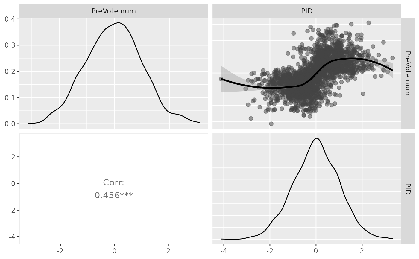
A plot matrix to display the results of partial association analyses. Upper-triangle contains scatter-plot matrix between each pair of response variables. Lower-triangle contains the partial correlation coefficients adjusted by covariates.
Arguments
- x
The object in "PAsso" class that is generated by "PAsso" or "test".
- color
The color of points.
- shape
The shapre of points. For more details see the help vignette:
vignette("ggplot2-specs", package = "ggplot2")- size
The size of points. For more details see the help vignette:
vignette("ggplot2-specs", package = "ggplot2")- alpha
The value to make the points transparent. For more details see the help vignette:
vignette("ggplot2-specs", package = "ggplot2")- ...
Additional optional arguments to be passed onto.
Details
A pairwise plot matrix reveals the partial association between ordinal variables.
All the plots are based on surrogate residuals generated from "resides" function.
Graphics are designed based on ggplot2 and "GGally".
Examples
data(ANES2016)

summary(ANES2016)
#>       age           edu.year      education     income.num
#>  Min.   :18.00   Min.   : 8.00   BAdeg :579   Min.   :  5.0
#>  1st Qu.:37.00   1st Qu.:14.00   CCdeg :327   1st Qu.: 37.5
#>  Median :53.00   Median :15.00   Coll  :447   Median : 67.5
#>  Mean   :51.25   Mean   :15.52   HS    :307   Mean   : 81.9
#>  3rd Qu.:65.00   3rd Qu.:17.00   HSdrop: 70   3rd Qu.:105.0
#>  Max.   :90.00   Max.   :19.00   MAdeg :440   Max.   :250.0
#>                                  MS    : 18
#>                         income          PID            selfLR
#>  (21) 21. $80,000-$89,999  : 138   Min.   :1.000   Min.   :1.000
#>  (24) 24. $110,000-$124,999: 123   1st Qu.:2.000   1st Qu.:3.000
#>  (17) 17. $60,000-$64,999  : 116   Median :4.000   Median :4.000
#>  (15) 15. $50,000-$54,999  : 114   Mean   :3.947   Mean   :4.158
#>  (27) 27. $175,000-$249,999: 112   3rd Qu.:6.000   3rd Qu.:6.000
#>  (23) 23. $100,000-$109,999: 111   Max.   :7.000   Max.   :7.000
#>  (Other)                   :1474
#>     TrumpLR          ClinLR                PreVote      PreVote.num
#>  Min.   :1.000   Min.   :1.000   DonaldTrump   :1065   Min.   :0.0000
#>  1st Qu.:5.000   1st Qu.:1.000   HillaryClinton:1123   1st Qu.:0.0000
#>  Median :6.000   Median :2.000                         Median :0.0000
#>  Mean   :5.261   Mean   :2.415                         Mean   :0.4867
#>  3rd Qu.:6.000   3rd Qu.:3.000                         3rd Qu.:1.0000
#>  Max.   :7.000   Max.   :7.000                         Max.   :1.0000
#>
#>  WeightforPreVote
#>  Min.   :0.1100
#>  1st Qu.:0.5759
#>  Median :0.8071
#>  Mean   :0.9482
#>  3rd Qu.:1.1347
#>  Max.   :6.8139
#>

PAsso_2v <- PAsso(responses = c("PreVote.num", "PID"),
                 adjustments = c("income.num", "age", "edu.year"),
                 data = ANES2016)

plot(PAsso_2v)